When I first started to learn about machine learning, specifically supervised learning, I eventually felt comfortable with taking some input $\mathbf{X}$, and determining a function $f(\mathbf{X})$ that best maps $\mathbf{X}$ to some known output value $y$. Separately, I dove a little into time series analysis and thought of this as a completely different paradigm. In time series, we don’t think of things in terms of features or inputs; rather, we have the time series $y$, and $y$ alone, and we look at previous values of $y$ to predict future values of $y$.
Still, I often wondered, “Where does machine learning end and time series begin?”. Or, “How do I use “features” in time series?”. I guess if you can answer these questions really well, then you’re in for making some money in finance. Or not. I have no idea - I really know nothing about that world.
I have had trouble answering these questions, in no small part due to the common difficulty of dealing with domain-specific vocabulary. I find myself having to internally translate time series concepts into “familiar” machine learning concepts. With this in mind, I would thus like to kick off a series of blog posts around analyzing time series data with the hopes of presenting these concepts in a familiar form. Due to the ubiquity of scikit-learn, I’ll assume that the scikit-learn API constitutes a familiar form.
To start the series off, in this post I’ll introduce a time series dataset that I’ve gathered. I’ll then walk through how we can turn the time series forecasting problem into a classic linear regression problem.
Let’s find a y(t)
The requirements for a suitable time series dataset are fairly minimal: We need some quantity that changes with time. Ideally, our data set could exhibit some patterns such that we can learn some things like seasonality and cyclic behavior. Thankfully, I’ve got just the dataset!
This is where you groan because I say that the dataset is related to the Citi Bike NYC bikeshare data. Everybody writes about this damn dataset, and it’s been beaten to death. Well, I agree, but hear me out. I’m not using the same dataset that everybody else uses. The typical Citi Bike dataset consists of all trips taken on the bikes. My dataset looks at the the number of bikes at each station as a function of time. Eh?
I started collecting this data about a year and a half ago because I was dealing with a common, frustrating scenario. I would check the Citi Bike app to make sure that there would be docks available at the station by my office before I left my apartment in the morning. However, by the time I rode to the office station, all the docks would have filled up, and I’d then have to go searching for a different station at which to dock the bike. Ideally, my app should tell me that, even though there are 5 docks available right now, they will likely be unavailable by the time I get there.
I wanted to collect this data and predict this myself. I still haven’t done that, but hopefully we will later on in this blog series. In the meantime, since 9/18/2016, I pinged the Citi Bike API every 2 minutes to collect how many bikes and docks are available at every single citi bike station in NYC. In the spirit of not planning ahead, this all just runs on a cron job on a t2.micro EC2 instance backed by a Postgres database that is running locally on the same instance. There are some gaps in the data due to me occasionally running out of hard drive space on the instance. The code for this lives in this repo, and I’ve stored more than 200 million records.
For more information about this dataset, I wrote a brief post on Making Dia.
For our purposes today, I am going to focus on a single time series from this data. The time series consists of the number of available bikes at the station at East 16th St and 5th Ave (i.e. the closest one to my apartment) as a function of time. Specifically, time is indexed by the last_communication_time. The Citi Bike API seems to update its values with random periodicity for different stations. The last_communication_time corresponds to the last time that the Citi Bike API talked to the station at the time of me querying.
We’ll start by reading the data in with pandas. Pandas is probably the preferred library to use for exploring time series data in Python. It was originally built for analyzing financial data which is why it shines so well for time series. For an excellent resource on time series modeling in pandas, check out Tom Aguspurger’s post in his Modern Pandas series. While I found that post to be extremely helpful, I am more interested in why one does certain things with time series as opposed to how to do these things.
My bike availability time series is in the form of a pandas Series object and is stored as a pickle file. Often, one does not care about the order of the index in Pandas objects, but, for time series, you will want to sort the values in chronological order. Note that I make sure the index is a sorted pandas DatetimeIndex.
%config InlineBackend.figure_format = 'retina'

import datetime
import time

import matplotlib as mpl
import matplotlib.pyplot as plt
import numpy as np
import pandas as pd

plt.ion()

mpl.rcParams['axes.labelsize'] = 20
mpl.rcParams['axes.titlesize'] = 24
mpl.rcParams['figure.figsize'] = (8, 4)
mpl.rcParams['xtick.labelsize'] = 14
mpl.rcParams['ytick.labelsize'] = 14
mpl.rcParams['legend.fontsize'] = 14
# Load and sort the dataframe.

df = pd.read_pickle('home_dat_20160918_20170604.pkl')
df.set_index('last_communication_time', inplace=True)
df.index = pd.to_datetime(df.index)
df.sort_index(inplace=True)
df.head()
| execution_time | available_bikes | available_docks | id | lat | lon | st_address | station_name | status_key | status_value | test_station | total_docks | |
|---|---|---|---|---|---|---|---|---|---|---|---|---|
| last_communication_time | ||||||||||||
| 2016-09-18 16:58:36 | 2016-09-18 16:59:51 | 4 | 43 | 496 | 40.737262 | -73.99239 | E 16 St & 5 Ave | E 16 St & 5 Ave | 1 | In Service | f | 47 |
| 2016-09-18 16:58:36 | 2016-09-18 17:01:47 | 4 | 43 | 496 | 40.737262 | -73.99239 | E 16 St & 5 Ave | E 16 St & 5 Ave | 1 | In Service | f | 47 |
| 2016-09-18 17:02:29 | 2016-09-18 17:03:42 | 7 | 40 | 496 | 40.737262 | -73.99239 | E 16 St & 5 Ave | E 16 St & 5 Ave | 1 | In Service | f | 47 |
| 2016-09-18 17:02:29 | 2016-09-18 17:05:48 | 7 | 40 | 496 | 40.737262 | -73.99239 | E 16 St & 5 Ave | E 16 St & 5 Ave | 1 | In Service | f | 47 |
| 2016-09-18 17:07:06 | 2016-09-18 17:07:44 | 7 | 40 | 496 | 40.737262 | -73.99239 | E 16 St & 5 Ave | E 16 St & 5 Ave | 1 | In Service | f | 47 |
# Pick out our time series object
# and fix it to a 5-min sampling period

y = df.available_bikes
y.index.name = 'time'
y = y.resample('5T').last()
y.head()
time
2016-09-18 16:55:00     4.0
2016-09-18 17:00:00     7.0
2016-09-18 17:05:00     6.0
2016-09-18 17:10:00     5.0
2016-09-18 17:15:00    10.0
Freq: 5T, Name: available_bikes, dtype: float64
ax = y.plot();
ax.set_ylabel('# Bikes');
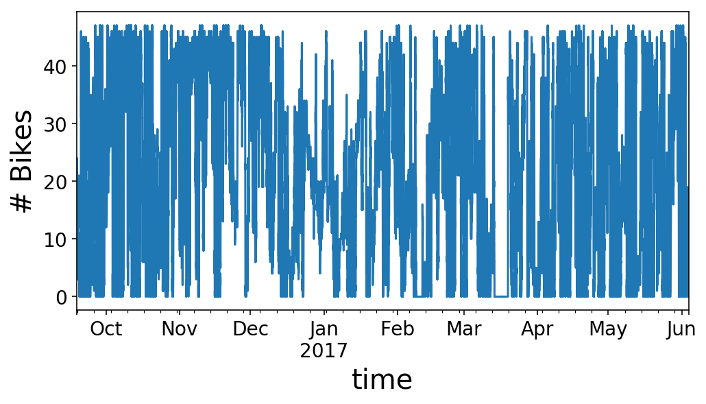
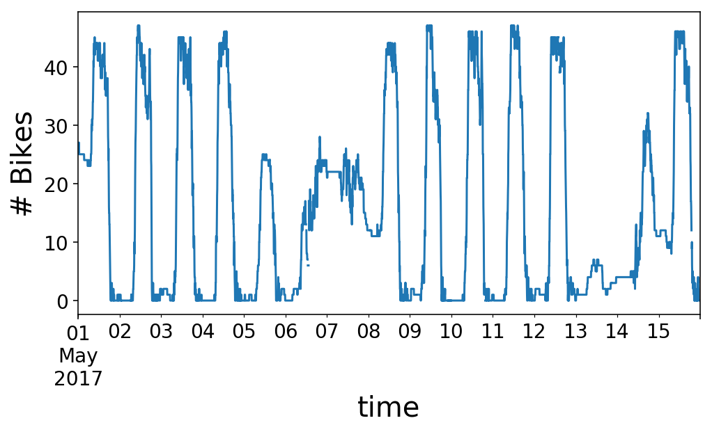
As you can see, our time series looks like kind of a mess. We can zoom in on the first half of May to get a better view of what’s going on. It looks like we have a regular rise and fall of our available bikes that happens each day with somewhat different behavior on the weekends (5/1 was a Monday, and 5/6 was a Saturday, in case you’re wondering).
y.loc['2017-05-01':'2017-05-15'].plot();
plt.ylabel('# Bikes');
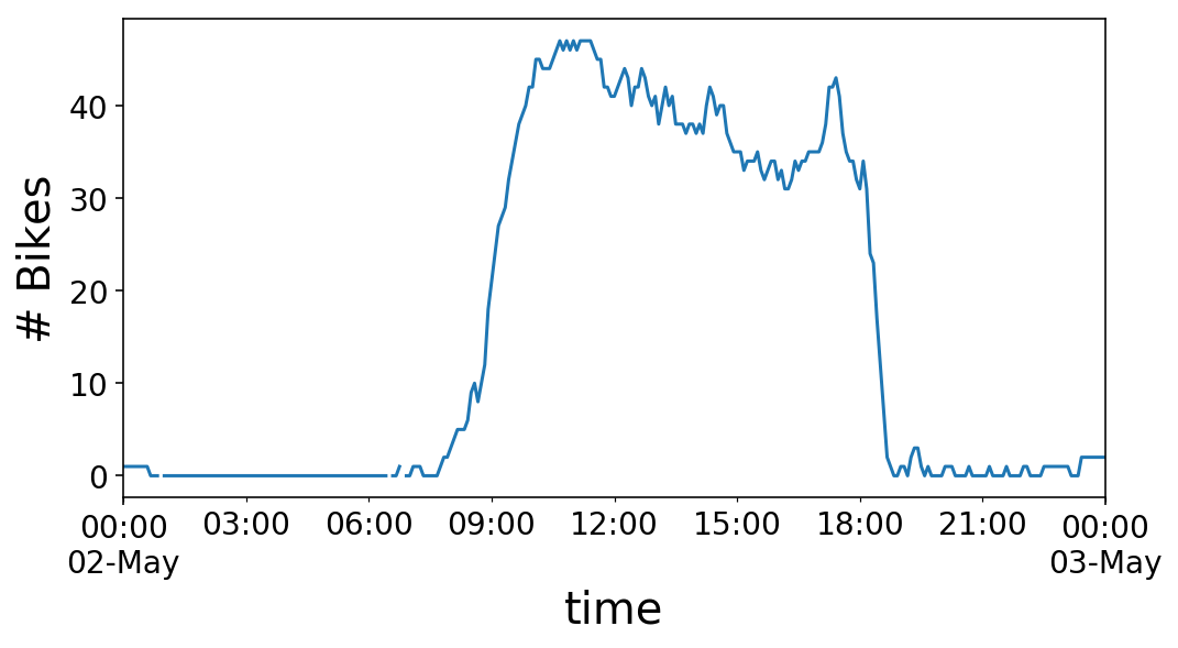
If we zoom in on a single day, we see that the number of bikes at the station rises in the morning, around 9 AM, and then plummets in the evening, around 6 PM. I’d call this a “commuter” station. There are a lot of offices around this station, so many people ride to the station in the morning, drop a bike off, and then pick up a bike in the evening and ride away. This works out perfectly for me, as I get to take the reverse commute.
y.loc['2017-05-02 00:00:00':'2017-05-03 00:00:00'].plot();
plt.ylabel('# Bikes');
<> Input <> Output <> Input <> Output <>
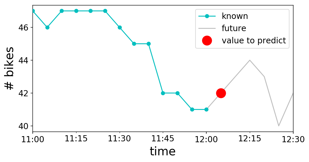
Excellent, we have our time series. What now? Let’s think about what we actually want to do with it. To keep things simple, let’s say that we want to be able to predict the next value in the time series. As an example, if it was noon (i.e. 12:00 PM) on May 2nd, we would be trying to predict the number of bikes available at 12:05 PM, since our time series is in periods of 5 minutes. Visually, this looks like the following:
known = y.loc['2017-05-02 11:00:00':'2017-05-02 12:00:00']
unknown = y.loc['2017-05-02 12:00:00':'2017-05-02 12:30:00']
to_predict = y.loc['2017-05-02 12:05:00':'2017-05-02 12:06:00']

fig, ax = plt.subplots();
known.plot(ax=ax, c='c', marker='o', zorder=3);
unknown.plot(ax=ax, c='grey', alpha=0.5);
to_predict.plot(ax=ax, c='r', marker='o', markersize=16,
                linestyle='');

ax.legend(['known', 'future', 'value to predict']);
ax.set_ylabel('# bikes');
Now that we have framed our problem in terms of what we know and what we want to predict, we walk back from whence we came towards ol’ machine learning. In time series, instead of creating a bunch of features to input into our model, we instead use the historical, known values of our time series as “features” to input into a model. The future value of the time series that we want to predict is then our target label. Mathematically, we will think of $\textbf{X}$ as our “feature matrix” or “design matrix” from machine learning. We would like to approximate $y$ with $\hat{y}$, and we’ll learn a function $\hat{y} = f(\textbf{X})$ in order to do this. Our $\textbf{X}$ matrix consists of previous values of $y$, our time series. Thus, at some point in time $t$,
$$\mathbf{X}_{t} = \mathbf{y}_{t^{\prime}\lt t}$$
where I have somewhat abused notation via the following
$$\mathbf{y}_{t^{\prime}\lt t} \equiv \big(y_{1}, y_{2}, \ldots, y_{t-2}, y_{t-1} \big)$$
where the portion on the right denotes a vector. Consequently, if we want to predict $y$ at time $t$, then it will be
$$\hat{y}_{t} = f(\mathbf{X}_{t})$$ $$\hat{y}_{t} = f(\mathbf{y}_{t^{\prime}\lt t-1})$$
Note that we cannot use future values to also predict the future. This is why we have to use the $t-1$ value of $\textbf{X}$ to predict $y_{t}$. In our graph from above, $t$ is 12:05 PM, the time that we are trying to predict. $\textbf{X}_{t-1}$ is the “known” cyan curve, and $y_{t}$ is the “value to predict” red marker.
Building the X matrix
Now that we’re able to think of time series in the comfortable form of $\hat{y} = f(\mathbf{X})$, how do we build up the full design matrix $\textbf{X}$? We would like to think of things in the scikit-learn paradigm, where we want to fit a design matrix $\textbf{X}$ in which each column is a feature dimension and each row is a separate “sample” or “data point”. In our case, each column of $\textbf{X}$ will map to a previous value of $y$. We then have to think of how to build multiple samples.
Before we build samples, though, let’s introduce the concept of a window. Recall that $\mathbf{X}_{t} = \mathbf{y}_{t^{\prime}\lt t}$. We could use all values of $y$ up until time $t$, but this would quickly get unwieldy for large time series. Instead, we can consider some finite number of $y$ values preceding $t$. This finite range is our window. For a window size $w$, $\mathbf{X}_{t} = \big(y_{t-w}, y_{t-w+1},\ldots, y_{t-2}, y_{t-1} \big)$.
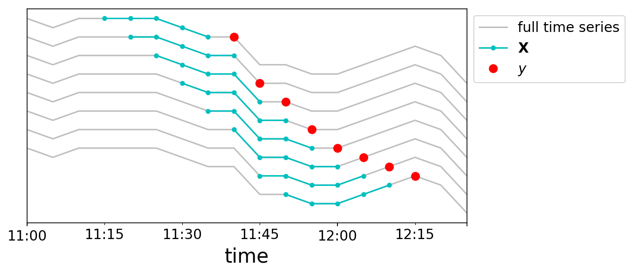
We can now build up our data samples. We will chop our time series into a bunch of samples where each $\mathbf{X}_{t}$ is a length $w$ vector, and our targets are $y_{t}$. We’ll again do this graphically. We take a window size of 5, and create 8 data points near noon on May 2nd. Each line plotted corresponds to a different row in our $\mathbf{X}$ matrix, and the lines are vertically offset for clarity.
fig, ax = plt.subplots();

start = np.where(y.index == '2017-05-02 11:00:00')[0][0]
middle = np.where(y.index == '2017-05-02 12:15:00')[0][0]
end = np.where(y.index == '2017-05-02 12:30:00')[0][0]

window = 5

for i in range(8):

    full = y.iloc[start:end]
    train = y.iloc[middle - i - window:middle - i ]
    predict = y.iloc[middle - i:middle - i + 1]

    (full + 2*i).plot(ax=ax, c='grey', alpha=0.5);
    (train + 2*i).plot(ax=ax, c='c', markersize=4,
                       marker='o')
    (predict + 2*i).plot(ax=ax, c='r', markersize=8,
                         marker='o', linestyle='')


ax.get_yaxis().set_ticks([]);
ax.legend(['full time series',
           '$\mathbf{X}$',
           '$y$'],
          bbox_to_anchor=(1, 1));
Just when I thought I was out, linear regression pulls me back in
We are now capable of building up a dataset in an analogous format to how we conventionally think about machine learning problems. Let’s say that we come up with some simple, linear model. We would like to learn some “feature weights” $\mathbf{a}$, such that
$$\mathbf{X}\mathbf{a} = \hat{\mathbf{y}}$$
Recall the shape of $\mathbf{X}$. We have a row for each data sample that we have created. For a time series of length $t$, and a window size of $w$, then we will have $t - w$ rows. The number of columns in $\textbf{X}$ is $w$. Consequently, $\textbf{a}$ will be a length-$w$ column vector. Putting it all together in matrix form looks like
$$ \begin{bmatrix} y_{0} & y_{1} & y_{2} & \dots & y_{w - 1} \cr y_{1} & y_{2} & y_{3} & \dots & y_{w} \cr \vdots & \vdots & \vdots & \ddots & \vdots \cr y_{t - 2 - w} & y_{t - 1 - w} & y_{t - w} & \dots & y_{t - 2} \cr y_{t - 1 - w} & y_{t - w} & y_{t - w + 1} & \dots & y_{t - 1} \cr \end{bmatrix} \begin{bmatrix} a_{0} \cr a_{1} \cr \vdots \cr a_{w-2} \cr a_{w-1} \end{bmatrix} = \begin{bmatrix} \hat{y}_{w} \cr \hat{y}_{w + 1} \cr \vdots \cr \hat{y}_{t - 1} \cr \hat{y}_{t} \end{bmatrix}$$
How could we learn these feature weights $\textbf{a}$? Ordinary Linear Regression shall do just fine. This means that our loss function looks like
$$\frac{1}{t-w}\sum\limits_{i=w}^{i=t}\big(y_{i} - \hat{y}_{i}\big)^{2}$$
We’re then free to minimize however we want. We’ll use scikit-learn for convenience:
#Build our matrices

window = 5
num_samples = 8
X_mat = []
y_mat = []
for i in range(num_samples):
    # Slice a window of features
    X_mat.append(y.iloc[middle - i - window:middle - i].values)
    y_mat.append(y.iloc[middle - i:middle - i + 1].values)

X_mat = np.vstack(X_mat)
y_mat = np.concatenate(y_mat)

assert X_mat.shape == (num_samples, window)
assert len(y_mat) == num_samples
from sklearn.linear_model import LinearRegression
from sklearn.metrics import r2_score

lr = LinearRegression(fit_intercept=False)
lr = lr.fit(X_mat, y_mat)
y_pred = lr.predict(X_mat)
fig, ax = plt.subplots(figsize=(6, 6));

ax.scatter(y_pred, y_mat);

one_to_one = np.arange(y_mat.min()-2, y_mat.max()+2)
ax.plot(one_to_one, one_to_one, c='r', linestyle='--');

ax.set_xlim((one_to_one[0], one_to_one[-1]));
ax.set_ylim((one_to_one[0], one_to_one[-1]));
ax.set_xlabel('Predicted');
ax.set_ylabel('True');
ax.set_title(f'$R^{2}$ = {r2_score(y_mat, y_pred):3.2f}');
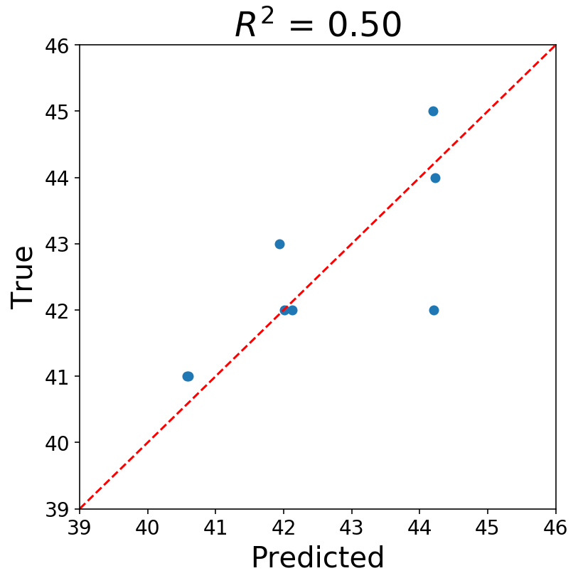
Now you can ask yourself if what we’ve done is okay, and the answer should probably be “No”. I’m assuming most statisticians would be extremely uncomfortable right now. There’s all sorts of issues, but, first and foremost, our data points are most assuredly not IID. Most of the statistical issues with the above roll up into the concept that the data must be stationary before running a regression. Also, our time series consists of strictly integer values, and using continuous models seems suspect to me.
Nevertheless, I’m fine with what we did. The goal of the above was to show that it is possible to cast a time series problem into a familiar format.
By the way, what we have done is defined and solved an autoregressive model which is the first two letters in the infamous ARIMA family of models.
Now that we’ve seen how to turn a time series problem into a typical supervised learning problem, one can easily add features to the model as extra columns in the design matrix, $\mathbf{X}$. The tricky part about time series is that, because you’re predicting the future, you must know what the future values of your features will be. For example, we could add in a binary feature indicating whether or not there is rain into our bike availablility forecaster. While this could potentially be useful for increasing accuracy on the training data, we would need to be able to accurately forecast the weather in order to forecast the time series far into the future, and we all know how hard weather forecasting is! In general, building training and test data for features that change with time is difficult, as it can be easy to leak information from the future into the past.
Lastly, I would also like to point out that, while we chose to use Linear Regression as our model, we could have used any other type of model, such as a random forest or neural network.
In the next post, I’ll walk through how we can correctly build up a design matrix, and we’ll take on the task of forecasting bike availability.